As with selection statements loops can be nested. Care should be taken when nesting loops as their inclusion in a program decreases the readability of the code. Unless we are undertaking some fairly trivial nesting it is normally better to encode the nested loops in the form of procedures or functions called from the "parent" loop.
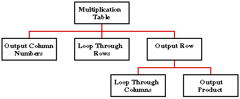
Produce an Ada program that outputs a 12x12 table such that the intersections of coordinates represent the product of the coordinates, i.e. a 12x12 multiplication table.
A top down analysis of the problem is given below.

We will implement this using a single procedure:
| NAME | DESCRIPTION | TYPE | RANGE |
|---|---|---|---|
| START_VALUE | Global constant | INTEGER | 1 |
| END_VALUE | Global constant | INTEGER | 12 |
An appropriate Nassi-Schneiderman design is given below.
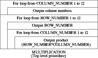
The encoding of the above design is as follows:
-- MULTIPLICATION
-- 16 September 1997
-- Frans Coenen
-- Dept Computer Science, University of Liverpool

with TEXT_IO;
use TEXT_IO;

procedure MULTIPLICATION is
    package INTEGER_INOUT is new INTEGER_IO(INTEGER);
    use INTEGER_INOUT;
    START_VALUE : constant INTEGER := 1;
    END_VALUE   : constant INTEGER := 12;
begin
-- Output top line of coordinates
    PUT("     |");
    for COLUMN_NUMBER in START_VALUE..END_VALUE loop
                PUT(COLUMN_NUMBER, WIDTH=>4);
    end loop;
    NEW_LINE;
    PUT_LINE("-----+-------------------------------------------------");
-- Output table entries
    for ROW_NUMBER in START_VALUE..END_VALUE loop
        PUT(ROW_NUMBER, WIDTH=>4);
        PUT(" |");
        for COLUMN_NUMBER in START_VALUE..END_VALUE loop
            PUT(ROW_NUMBER*COLUMN_NUMBER, WIDTH=>4);
            end loop;
            NEW_LINE;
    end loop;
    NEW_LINE;
end MULTIPLICATION;
There are no input values or other means whereby the user can influence the operation of the program, therefore a single rum through will suffice to test the operation of the program.
     |   1   2   3   4   5   6   7   8   9  10  11  12
-----+-------------------------------------------------
   1 |   1   2   3   4   5   6   7   8   9  10  11  12
   2 |   2   4   6   8  10  12  14  16  18  20  22  24
   3 |   3   6   9  12  15  18  21  24  27  30  33  36
   4 |   4   8  12  16  20  24  28  32  36  40  44  48
   5 |   5  10  15  20  25  30  35  40  45  50  55  60
   6 |   6  12  18  24  30  36  42  48  54  60  66  72
   7 |   7  14  21  28  35  42  49  56  63  70  77  84
   8 |   8  16  24  32  40  48  56  64  72  80  88  96
   9 |   9  18  27  36  45  54  63  72  81  90  99 108
  10 |  10  20  30  40  50  60  70  80  90 100 110 120
  11 |  11  22  33  44  55  66  77  88  99 110 121 132
  12 |  12  24  36  48  60  72  84  96 108 120 132 144
Example Problem Multiplication Report.
An alternative implementation might comprise three procedures:
| NAME | DESCRIPTION | TYPE | RANGE |
|---|---|---|---|
| START_VALUE | Global constant | INTEGER | 1 |
| END_VALUE | Global constant | INTEGER | 12 |
| NAME | DESCRIPTION | TYPE | RANGE |
|---|---|---|---|
| ROW_NUMBER | Local variable | INTEGER | Default |
Note that this approach dispenses with the need to include nested loops. Appropriate Nassi-Schneiderman charts for these procedures are given below.
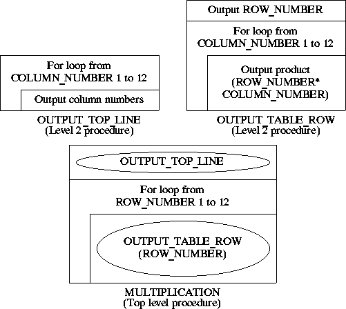
The implementation will be as follows:
-- MULTIPLICATION
-- 16 September 1997
-- Frans Coenen
-- Dept Computer Science, University of Liverpool

with TEXT_IO;
use TEXT_IO;

procedure MULTIPLICATION is
    package INTEGER_INOUT is new INTEGER_IO(INTEGER);
    use INTEGER_INOUT;
    START_VALUE : constant INTEGER := 1;
    END_VALUE   : constant INTEGER := 12;

    -----------------------------------------------------------------------
    -- OUTPUT TOP LINE
    procedure OUTPUT_TOP_LINE is
    begin
        PUT("     |");
        for COLUMN_NUMBER in START_VALUE..END_VALUE loop
            PUT(COLUMN_NUMBER, WIDTH=>4);
        end loop;
        NEW_LINE;
        PUT_LINE("-----+------------------------------------------------");
    end OUTPUT_TOP_LINE;
    -----------------------------------------------------------------------
    -- OUTPUT TABLE ROW
    procedure OUTPUT_TABLE_ROW (ROW_NUMBER: INTEGER) is
    begin
        PUT(ROW_NUMBER, WIDTH=>4);
        PUT(" |");
        for COLUMN_NUMBER in START_VALUE..END_VALUE loop
            PUT(ROW_NUMBER*COLUMN_NUMBER, WIDTH=>4);
            end loop;
            NEW_LINE;
    end OUTPUT_TABLE_ROW;
    -----------------------------------------------------------------------

-- TOP LEVEL PROCEDURE
begin
-- Output top line of coordinates
    OUTPUT_TOP_LINE;
-- Output table entries
    for ROW_NUMBER in START_VALUE..END_VALUE loop
            OUTPUT_TABLE_ROW(ROW_NUMBER);
    end loop;
    NEW_LINE;
end MULTIPLICATION;
To produce random numbers using a computer we generate a series of numbers:
N0, N1, N2, N3, ...that appear to be random. The most common equation used to generate such a series is:
N+1 = KxN mod M
where mod is the modulus operator, K and M are constants, M is the current term (random number) and N+1 is the following term. This equation requires a start term (N0), often referred to as the seed, after which subsequent terms can be generated. To ensure realistic operation of the equation appropriate values for K and M. For example if N0 = 3, K = 5 and M = 4 all the terms will be equivalent to 3 (5x3 mod 4 = 3). Theories exist on the best choice of values for K and M, Skansholm (1997) suggests:
K = 5^5 = 3125
M = 2^13 = 8192
and a seed with an odd number value within the range of 1..M-1 (i.e. 1..8191). This will then produce a series of "random" numbers within the range 1..M-1 (i.e. 1..8191). If we wished to produce random numbers between say 0..99 or 0..9 inclusive we would have to apply the corrections:
100/8191 or 10/8191
Develop and produce a program that generates a series of random numbers between 0 and 99 inclusive until the number 50 is generated. Use the equation:
N+1 = 3125xN mod 8192
where:
Note that to start the series we require an initial value for N which must be an odd number between 1 and 1891. Note also that the equation will produce terms ("random numbers") within the range 1 to 8191 therefore to produce random numbers within the range 0 to 99 inclusive we must multiply the result by 100/8191.
A top down analysis of the problem is given below.

The above can be implemented using the following procedures/functions
| NAME | DESCRIPTION | TYPE | RANGE |
|---|---|---|---|
| M_CONSTANT | Global constant | INTEGER | 8192 |
| K_CONSTANT | Global constant | INTEGER | 3125 |
| RAND_NUM | Global variable | NATURAL | Default |
| TERM | Global variable | NATURAL | Default |
| NAME | DESCRIPTION | TYPE | RANGE |
|---|---|---|---|
| SEED | local input variable | POSITIVE | 1..M_CONSTANT-1 |
Appropriate Nassi-Schneiderman charts are given below.
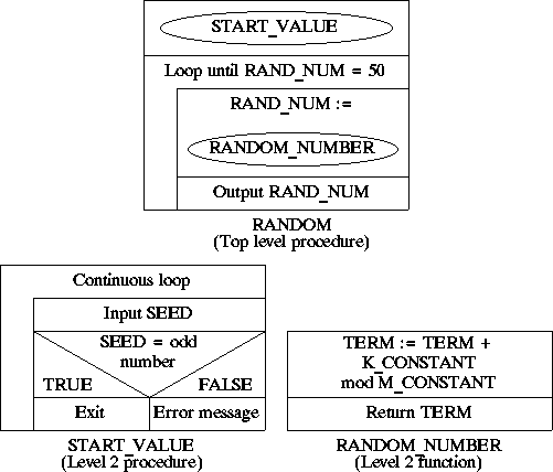
The encoding of the above design is as follows:
-- RANDOM NUMBER GENERATOR
-- 16 September 1997
-- Frans Coenen
-- Dept Computer Science, University of Liverpool

with TEXT_IO;
use TEXT_IO;

procedure RANDOM is
    package INTEGER_INOUT is new INTEGER_IO(INTEGER);
    use INTEGER_INOUT;
    package FLOAT_INOUT is new FLOAT_IO(FLOAT);
    use FLOAT_INOUT;
    M_CONSTANT : constant := 8192;     -- 2**13
    K_CONSTANT : constant := 3125;     -- 5**5
    RAND_NUM   : NATURAL  := 0;
    TERM       : NATURAL;

------------------------------------------------------------
-- START VALUE PROCEDURE
    procedure START_VALUE is
        SEED: POSITIVE range 1..M_CONSTANT-1;
    begin
        loop
    -- Output request to user and get SEED
            PUT("Enter seed (odd number within the range 1 to ");
            PUT(M_CONSTANT-1, WIDTH=>4);
            PUT_LINE("): ");
            GET(SEED);
    -- Check seed (seed must be an odd number
            if SEED rem 2 = 1 then
                TERM := SEED;
                exit;
            else
                PUT("Invalid seed: ");
                PUT(SEED);
                PUT_LINE(", try again");
                NEW_LINE;
            end if;
        end loop;
        NEW_LINE;
    end START_VALUE;

----------------------------------------------------------
-- RANDOM NUMBER
    function RANDOM_NUMBER return NATURAL is
    begin
        TERM := TERM * K_CONSTANT mod M_CONSTANT;
        RETURN(TERM);
    end RANDOM_NUMBER;

----------------------------------------------------------
-- TOP LEVEL
begin
    START_VALUE;
    while RAND_NUM /= 50 loop
        RAND_NUM := RANDOM_NUMBER*100/8191;
        PUT(RAND_NUM, WIDTH=>4);
    end loop;
    NEW_LINE;
end RANDOM;
BVA testing: We should test the input range values for the variable SEED using a set of BVA test cases of the form given in the table below.
| TEST CASE | EXPECTED RESULT |
|---|---|
| SEED | OUTPUT |
| 0 | CONSTRAINT_ERROR |
| 2 | Invalid seed |
| 8190 | Invalid seed |
| 8192 | CONSTRAINT_ERROR |
Limit testing: A set of limit test cases is given in the table below.
| TEST CASE | EXPECTED RESULT |
|---|---|
| SEED | OUTPUT |
| 1 | Sequence of random numbers |
| 8191 | Sequence of random numbers |
| TEST CASE | EXPECTED RESULT |
|---|---|
| SEED | OUTPUT |
| 495 | Sequence of random numbers |
Arithmetic testing: Arithmetic testing dictates test cases using a negative, zero and positive sample values for the input variables. In this case there is only one input variable, a negative value is precluded by its type definition and we have already incorporated a zero sample value in the limit test cases given in Table 6. We therefore only need to define a single arithmetic test case involving a positive sample value (see table right).
Path and loop testing: We should test both paths through the START_VALUE procedure using an odd and an even value. However, this has already been taken into consideration by the preceding black box test cases. The loop is a variable count loop which cannot be influenced by the user in a predictable manner. Therefore loop testing is not required in this case either.
This should also be done.
Example Problem Random Number Generator Report.
Created and maintained by Frans Coenen. Last updated 11 October 1999