Dynamic Programming

This paradigm is most often applied in the construction of algorithms to solve a certain class of

Optimisation Problem

That is: problems which require the minimisation or maximisation of some measure.

One disadvantage of using Divide-and-Conquer is that the process of recursively solving separate sub-instances can result in the same computations being performed repeatedly since identical sub-instances may arise.

The idea behind dynamic programming is to avoid this pathology by obviating the requirement to calculate the same quantity twice.

The method usually accomplishes this by maintaining a table of sub-instance results.

Dynamic Programming is a

Bottom-Up Technique

in which the smallest sub-instances are explicitly solved first and the results of these used to construct solutions to progressively larger sub-instances.

In contrast, Divide-and-Conquer is a

Top-Down Technique

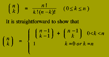
which logically progresses from the initial instance down to the smallest sub-instances via intermediate sub-instances. We can illustrate these points by considering the problem of calculating the Binomial Coefficient, "n choose k", i.e.

Using this relationship, a rather crude Divide-and-Conquer solution to the problem of calculating the Binomial Coefficient `n choose k' would be:

function bin_coeff (n : integer;
                                k : integer)
                                return integer is
   begin
      if k = 0 or k = n then
         return 1;
      else
         return 
         bin_coeff(n-1, k-1) + bin_coeff(n-1, k);
      end if;
   end bin_coeff;

By contrast, the Dynamic Programming approach uses the same relationship but constructs a table of all the (n+1)*(k+1) binomial coefficients `i choose j' for each value of i between 0 and n, each value of j between 0 and k.

These are calculated in a particular order:

• First the table entries corresponding to the coefficients `i choose 0' and `1 choose 1' are fixed to the value 1.
• The remaining table entries corresponding to the binomial coefficient `i choose j' are calculated in increasing order of the value of i+j.

(i-1)+(j-1) < (i-1)+j < i+j

The Dynamic Programming method is given by:

function bin_coeff (n : integer;
                                k : integer)
                                return integer is
type table is array (0..n, 0..k) of integer;
bc : table;
i, j, k : integer;
sum : integer;
begin
   for i in 0..n loop
     bc(i,0) := 1;
   end loop;
   bc(1,1) := 1;
   sum := 3; i := 2; j := 1;
   while sum <= n+k loop
      bc(i,j) := bc(i-1,j-1)+bc(i-1,j);
      i := i-1; j := j+1;
      if i < j or j > k then
         sum := sum + 1;                     
         if sum <= n+1 then      
            i := sum-1; j := 1;            
         else                           
            i := n; j := sum-n;          
         end if;                      
      end if;                        
    end loop;
   return bc(n,k);
end bin_coeff;

The section of the function consisting of the lines:

if i < j or j > k then
   sum := sum + 1;                     
   if sum <= n+1 then      
      i := sum-1; j := 1;            
   else                           
      i := n; j := sum-n;          
   end if;                      
end if;                        

is invoked when all the table entries `i choose j', for which i+j equals the current value of sum, have been found. The if statement increments the value of sum and sets up the new values of i and j.

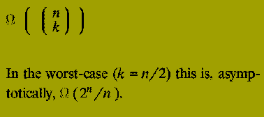
Now consider the differences between the two methods: The Divide-and-Conquer approach recomputes values, such as "2 choose 1", a very large number of times, particularly if n is large and k depends on n, i.e. k is not a constant.

It can be shown that the running time of this method is

Despite the fact that the algorithm description is quite simple (it is just a direct implementation of the relationship given) it is completely infeasible as a practical algorithm.

The Dynamic Programming method, since it computes each value "i choose j" exactly once is far more efficient. Its running time is O( n*k ), which is O( n^2 ) in the worst-case, (again k = n/2).

It will be noticed that the dynamic programming solution is rather more involved than the recursive Divide-and-Conquer method, nevertheless its running time is practical.

The binomial coefficient example illustrates the key features of dynamic programming algorithms.

• A table of all sub-instance results is constructed.
• The entries corresponding to the smallest sub-instances are initiated at the start of the algorithm.
• The remaining entries are filled in following a precise order (that corresponds to increasing sub-instance size) using only those entries that have already been computed.
• Each entry is calculated exactly once.
• The final value computed is the solution to the initial problem instance.
• Implementation is by iteration (never by recursion, even though the analysis of a problem may naturally suggest a recursive solution).

Example: Shortest Path

Input: A directed graph, G( V, E ), with nodes

             V  =  {1, 2 ,..., n }

and edges E as subset of VxV. Each edge in E has associated with it a non-negative length.

Output: An nXn matrix, D, in which D^(i,j) contains the length of the shortest path from node i to node j in G.

Informal Overview of Method

The algorithm, conceptually, constructs a sequence of matrices:

D0, D1 ,..., Dk ,..., Dn

For each k (with 1 < = k < = n), the (i, j) entry of Dk, denoted Dk( i,j ), will contain the Length of the shortest path from node i to node j when only the nodes

{ 1, 2, 3 ,..., k }

can be used as intermediate nodes on the path.

Obviously Dn = D.

The matrix, D0, corresponds to the `smallest sub-instance'. D0 is initiated as:

               0  if i=j
D0( i, j )  =  infinite  if (i,j) not in E
               Length(i,j)  if (i,j) is in E

Now, suppose we have constructed Dk, for some k < n.

How do we proceed to build D(k+1)?

The shortest path from i to j with only

{ 1, 2, 3 ,..., k, k+1 }

Either: Does not contain the node k+1.

Or: Does contain the node k+1.

In the former case:

                 D(k+1)( i, j )  =  Dk( i, j )

In the latter case:

            D(k+1)( i, j )  =  D-k( i, k+1 ) + D-k( k+1, j )

Therefore D(k+1)( i, j ) is given by

                       Dk(i,j)
               minimum 
                       Dk( i, k+1 ) + Dk( k+1, j )

Although these relationships suggest using a recursive algorithm, as with the previous example, such a realisation would be extremely inefficient.

Instead an iterative algorithm is employed.

Only one nXn matrix, D, is needed.

This is because after the matrix D(k+1) has been constructed, the matrix Dk is no longer needed. Therefore D(k+1) can overwrite Dk.

In the implementation below, L denotes the matrix of edge lengths for the set of edges in the graph G( V, E ).

type matrix is array (1..n, 1..n) of integer;
L : matrix
function shortest_path_length (L : matrix;
                                   n : integer) 
                                   return matrix is
D : matrix; -- Shortest paths matrix
begin
  -- Initial sub-instance
  D(1..n,1..n) := L(1..n,1..n); 
  for k in 1..n loop
    for i in 1..n loop
      for j in 1..n loop
        if D(i,j) > D(i,k) + D(k,j) then
           D( i,j ) := D(i,k) + D(k,j);
        end if;
      end loop;
    end loop;
  end loop;
  return D(1..n,1..n);
end shortest_path_length;

This algorithm, discovered by Floyd, clearly runs in time

O( n^3 )

Thus O( n ) steps are used to compute each of the n^2 matrix entries.

• Overview
• Introduction
• Divide-and-Conquer Algorithms
• The Greedy Method
• Backtracking and Search Techniques

PED Home Page