The most high level approach to defining range/precision is through explicit specification. This is supported by Ada. Examples of data item declarations where specific ranges and/or precision are defined:
A_VALUE: INTEGER range 0 .. 100;

SUMMER: INTEGER is digits 3;

X_VALUE, Y_VALUE; FLOAT is digits 4  range 0.0 .. 100.0;
Note that, where appropriate, precision (number of digits) must be specified before range. The specification of ranges and/or precisions for data items (at least with respect to Ada) facilitates automatic checking of values. This is especially useful where input variables are required to be within a specific range or of a certain precision.
Note: precision is not the same as requiring output to be to a certain number of decimal places.

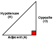
Given the length of the "opposite" (O) and "adjacent" (A) sides of a right angled triangle (see right) determine the "hypotenuse" (H) using Pythagoras theorem:
H^2 = O^2 + A^2
Assume sides are given as floating point numbers between 0.0 and 100.0 and that an accuracy of 4 decimal places is required
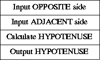
Using a top down analysis of the problem we can identify the operations shown below:

These operations are trivial enough to be encompassed by a single procedure:
| NAME | DESCRIPTION | TYPE | RANGE |
|---|---|---|---|
| OPPOSITE | Input variable | FLOAT | 0.0..100.0 |
| ADJACENT | Input variable | FLOAT | 0.0..100.0 |
| HYPOTENUSE | Global variable | FLOAT | 0.0..100.0 |

A Nassi-Shneiderman design is presented to the right.
The implementation of the design is as follows:
-- PYTHAGORAS
-- 6 August 1997
-- Frans Coenen
-- Dept Computer Science, University of Liverpool

with TEXT_IO, GENERIC_ELEMENTARY_FUNCTIONS;
use TEXT_IO;

procedure PYTHAGORAS is
        OPPOSITE, ADJACENT: FLOAT range 0.0..100.0;
        HYPOTENUSE: FLOAT;
        package FLOAT_INOUT is new FLOAT_IO(FLOAT);
        use FLOAT_INOUT;
        package MATH_FUNC is new GENERIC_ELEMENTARY_FUNCTIONS(FLOAT);
        use MATH_FUNC;
begin
-- Input opposite and adjacent side
        PUT_LINE("Input opposite and adjacent sides: ");
        GET(OPPOSITE);
        GET(ADJACENT);
-- Calculate hypotenuse
        HYPOTENUSE := OPPOSITE**2 + ADJACENT**2;
        HYPOTENUSE := SQRT(HYPOTENUSE);
-- Output hypotenuse
        PUT("Hypotenuse is: ");
        PUT(HYPOTENUSE, FORE=>3, AFT=>4, EXP=>0);
        NEW_LINE;
end PYTHAGORAS;
Notes:
package PACKAGE_NAME is new TEMPLATE_NAME(T);
use PACKAGE_NAME;
| TEST CASE | EXPECTED RESULT | |
|---|---|---|
| OPPOSITE | ADJACENT | HYPOTENUSE |
| -0.1 | * | CONSTRAINT_ERROR |
| 0.1 | -0.1 | CONSTRAINT_ERROR |
| 0.1 | 0.1 | 0.1414 |
| 99.9 | 99.9 | 141.2799 |
| 99.9 | 100.1 | CONSTRAINT_ERROR |
| 101.1 | * | CONSTRAINT_ERROR |
BVA Testing: When using "ranged" types it has been demonstrated that errors often occur at the boundaries of the input domain. It is for this reason that Boundary Value Analysis (BVA) has been developed as a testing technique. Boundary value analyses leads to a selection of test cases that exercise bounding values for data items. At its simplest this involves the derivation of test cases with values just above and just below the bounding values. Thus suitable boundary values for both OPPOSITE and ADJACENT are -0.1, 0.1, 99.9 and 100.1. An appropriate set of test cases is given in the table (above-right), where the * symbol indicates that no further input is required as we expect the code to fail after the previous input. Note that values for ADJACENT can only be tested given valid values for OPPOSITE.
| TEST CASE | EXPECTED RESULT | |
|---|---|---|
| OPPOSITE | ADJACENT | HYPOTENUSE |
| 0.0 | 0.0 | 0.0 |
| 0.0 | 100.0 | 100.0 |
| 100.0 | 0.0 | 100.0 |
| 100.0 | 100.0 | 141.4214 |
Limit testing: Ranged input data items should also be tested at their limits, i.e at their maximum and minimum permitted values. Two suitable test cases are given in the table to the right.
Data validation testing: We should also test the input with some spurious inputs, e.g. characters or too many inputs.
| TEST CASE | EXPECTED RESULT | |
|---|---|---|
| OPPOSITE | ADJACENT | HYPOTENUSE |
| 0.0 | 0.0 | 0.0 |
| 0.0 | 10.0 | 10.0 |
| 10.0 | 0.0 | 10.0 |
| 10.0 | 10.0 | 14.1421 |
Arithmetic testing Finally use straightforward arithmetic testing to test calculation. Normally this would require positive, zero and negative sample values for each input. However, in this case we need only to consider positive and zero values. A suitable set of test cases is given to the right.
Example Problem Pythagoras Report.
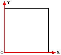
Design and implement an Ada program that determines the geographical distance between two points located on a geographic plane. The points are referenced using the standard {X,Y} Cartesian coordinate system founded on a 0 origin (see below). The geographic space of interest measures 100x100. X and Y Coordinates can therefore range from 0.0 to 100.0 inclusive. Distances should be determined to within 4 decimal places.

The distance between two two-dimensional points is given by:
DISTANCE = SQRT(X^22 + Y^2)
where X and Y respectively represent the difference between the pairs of x and y coordinates for the two points. To address this problem we can identify a number of operations as indicated by the top-down analysis presented below:

These operations are simple enough to be combined into a single procedure:
| NAME | DESCRIPTION | TYPE | RANGE |
|---|---|---|---|
| X1 | Input variable | FLOAT | 0.0..100.0 |
| Y1 | Input variable | FLOAT | 0.0..100.0 |
| X2 | Input variable | FLOAT | 0.0..100.0 |
| Y2 | Input variable | FLOAT | 0.0..100.0 |
| X_DIFF | Global variable | FLOAT | Default |
| Y_DIFF | Global variable | FLOAT | Default |
| DISTANCE | Global variable | FLOAT | Default |
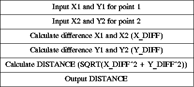
The design of this procedure is indicated by the Nassi-Shneiderman chart presented below.

-- 2D GEOGRAPHIC DISTANCE
-- 4 August 1997
-- Frans Coenen
-- Dept Computer Science, University of Liverpool

with TEXT_IO, GENERIC_ELEMENTARY_FUNCTIONS;
use TEXT_IO;

procedure GEO_DIST_2D is
        X1, Y1, X2, Y2: FLOAT range 0.0..100.0;
        X_DIFF, Y_DIFF, DISTANCE: FLOAT;
        package FLOAT_INOUT is new FLOAT_IO(FLOAT);
        use FLOAT_INOUT;
        package MATH_FUNC is new GENERIC_ELEMENTARY_FUNCTIONS(FLOAT);
        use MATH_FUNC;
begin
-- Input coordinates for point 1
        PUT_LINE("Input X and Y coordinates for point 1: ");
        GET(X1);
        GET(Y1);
-- Input coordinates for point 2
        PUT_LINE("Input X and Y coordinates for point 2: ");
        GET(X2);
        GET(Y2);
-- Calculate differences and distance
        X_DIFF := abs(X1-X2);
        Y_DIFF := abs(Y1-Y2);
        DISTANCE := SQRT(X_DIFF**2 + Y_DIFF**2);
-- Output distance
        PUT("Distance is: ");
        PUT(DISTANCE, FORE=>3, AFT=>4, EXP=>0);
        NEW_LINE;
end GEO_DIST_2D;
Note that the abs operator is a standard numeric operator which has one operand that can be of any arbitrary numeric type. The operator calculates the absolute value (or magnitude) of the operand, i.e. the operand itself if it is positive, and the negated operand if it is negative.
| TEST CASE | EXPECTED RESULT | |||
|---|---|---|---|---|
| X1 | Y1 | X2 | Y2 | DISTANCE |
| -0.1 | * | * | * | CONSTRAINT_ERROR |
| 100.1 | * | * | * | CONSTRAINT_ERROR |
| 0.1 | -0.1 | * | * | CONSTRAINT_ERROR |
| 99.9 | 100.1 | * | * | CONSTRAINT_ERROR |
| 0.1 | 0.1 | -0.1 | * | CONSTRAINT_ERROR |
| 99.9 | 99.9 | 100.1 | * | CONSTRAINT_ERROR |
| 0.1 | 0.1 | 0.1 | -0.1 | CONSTRAINT_ERROR |
| 99.9 | 99.9 | 99.9 | 100.1 | CONSTRAINT_ERROR |
| 0.1 | 99.9 | 99.9 | 0.1 | 141.1385 |
| 99.9 | 0.1 | 0.1 | 99.9 | 141.1385 |
BVA testing: Use BVA to test limits of input values. Appropriate values for X1, Y1, X2 and Y2 are -0.1, 0.1, 99.9 and 100.1 (just above and below the range limits). A set of test cases of this form is presented in the table to the right. The * symbol indicates where no further input is required as the code is expected to fail after the previous input.
Arithmetic testing: We should also carry out a set of numeric tests to check the workings of the arithmetic expressions. This could be done by generating a set of cases combining every possible combination of zero and positive sample input value (negative values are precluded in this case), i.e. 2 x 2 x 2 x 2 = 16 test cases. This would be rather tedious (and with more inputs impractical). We can reduce the amount of test cases required by investigating more closely the arithmetic operations we wish to check. There are three of these:
| 1. | Difference in X calculation | |
| 2. | Difference in Y calculation | |
| 3. | Pythagoras calculation | |
| SAMPLE VALUES | EXPECTED RESULT | ||||
|---|---|---|---|---|---|
| X1 | Y1 | X2 | Y2 | X_DIFF | Y_DIFF |
| 0 | 0 | 0 | 0 | 0 | 0 |
| +ve | +ve | 0 | 0 | +ve | +ve |
| 0 | 0 | +ve | +ve | +ve | +ve |
| +ve | +ve | +ve | +ve | +ve or 0 | +ve or 0 |
Commencing with the two difference calculations, we note that each is carried out independently from the other and thus can be tested simultaneously. Each should be tested with combinations of positive and zero sample values. An outline set of required test cases is given in the table to the right.
| SAMPLE VALUES | |
|---|---|
| X_DIFF | Y_DIFF |
| 0 | 0 |
| +ve | 0 |
| 0 | +ve |
| +ve | +ve |
Turning to the Pythagoras calculation this should be tested with sample values for X_DIFF and Y_DIFF comprising all possible combinations of zero and positive value (we cannot have a negative difference) as shown in the table to the right. Test cases required to check the difference calculation already identify the situation where both difference values are zero and both difference values are positive. We therefore simply need to derive two test cases where one or the other difference value is zero .
An appropriate set of numeric test cases with respect to the foregoing is given below. Note that we have reduced the number of arithmetic tests from 16 to 6. The first four of the following address the difference calculations and also the Pythagoras calculation where both differences are 0 and both differences are positive. The final two test cases are designed to exercise the Pythagoras calculation where one of the differences is zero and the other is positive (and vice-versa).
| TEST CASE | EXPECTED RESULT | |||
|---|---|---|---|---|
| X1 | Y1 | X2 | Y2 | DISTANCE |
| 0.0 | 0.0 | 0.0 | 0.0 | 0.0000 |
| 0.0 | 0.0 | 10.0 | 10.0 | 14.1421 |
| 10.0 | 10.0 | 0.0 | 0.0 | 14.1421 |
| 10.0 | 10.0 | 10.0 | 10.0 | 0.0000 |
| 20.0 | 10.0 | 20.0 | 30.0 | 20.0000 |
| 30.0 | 20.0 | 10.0 | 20.0 | 20.0000 |
Limit testing: We should also test the operations of the systems at the limits for the input data. Notionally there are four tests for each difference calculation covering every combination of 0.0 and 100.0 input. However, the above arithmetic test cases have considered the case where inputs are all 0.0. Therefore we only need to test combinations where one or both of the input is 100.0. An appropriate set of test cases is given in the table below.
| TEST CASE | EXPECTED RESULT | |||
|---|---|---|---|---|
| X1 | Y1 | X2 | Y2 | DISTANCE |
| 100.0 | 0.0 | 0.0 | 100.0 | 141.4214 |
| 0.0 | 100.0 | 100.0 | 0.0 | 141.4214 |
| 100.0 | 100.0 | 100.0 | 100.0 | 0.0000 |
Data validation: Finally we should carry out some tests using deliberately spurious data.
Example Problem 2D Geographic Distance Report.
Created and maintained by Frans Coenen. Last updated 11 October 1999